One More City, Zero Success: Stress-Testing Simulated Annealing

Introduction

In our last article, we introduced simulated annealing and watched it go head-to-head with brute force. For 11 cities, it found the same optimal path brute force needed 70 seconds for, in just 5 milliseconds, a 13,000x speedup. But we also flagged that this speed comes at a cost: annealing isn't guaranteed to find the perfect answer every time.

That leaves some open questions. How does annealing actually scale as the number of cities grows? Where does it start to break down? And what does its reliability really look like once we run it enough times to see the full picture?

That's what this article digs into.

After coming this far, it's natural to have one more important question in mind: as we increase the number of cities, how does the required number of iterations change? Does it grow exponentially, linearly, or in some other way?

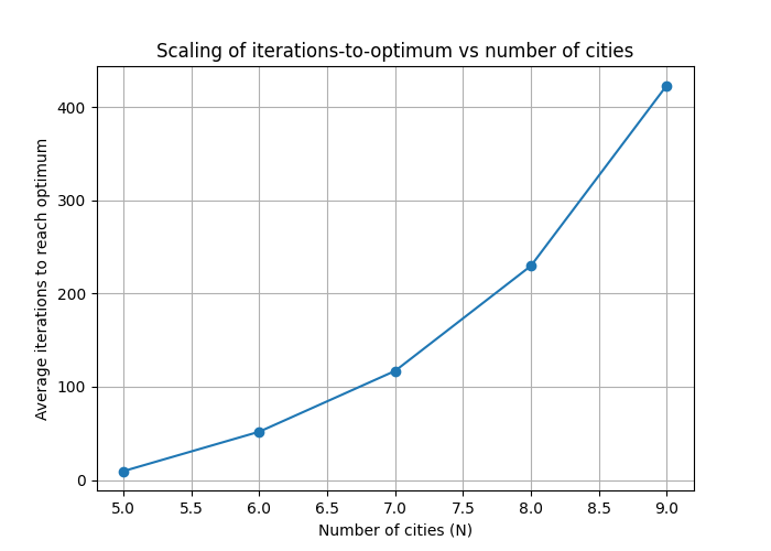
To answer this, we ran the algorithm 30 times (at a fixed number of iterations) for each problem size from 5 to 9 cities, counting only on successful runs in which the true optimal solution was found. While the "combinatorial explosion" makes simulating for many cities impractical, this range is enough to give us the gist of how the scaling properties of this algorithm.

The graphs shows how the average number of successful iterations (y-axis) scales as we increase the number of nodes (N) in our network (x-axis). It is clearly visible that the complexity is scaling more than just proportionally as we grow the number of cities in our problem.

1. The Scaling of Iterations: A Deeper Look

The graph shows our experiment's results, which indicates the exponential relationship between the number of cities and the average number of iterations required to find the optimal solution.

It's also interesting to note that the average number of iterations required to find the optimal solution for cities 5 through 9 was 166.36.

You may have noticed that in one of our earlier examples, the annealing algorithm found the perfect solution for 8 cities much faster than the brute-force method. However, as our deeper analysis shows, this isn't guaranteed to happen every time.

This isn't a discrepancy in the results; it's a feature of the algorithm itself. The outcome has an inherent probability that captures the true nature of this heuristic approach: it trades the certainty of perfection for a massive speed advantage.

A Deeper Dive into the Algorithm's Behavior

A little more depth wouldn't hurt, right? To truly understand the probabilistic nature of simulated annealing, we ran the algorithm 100 times for each problem size for 1000 iterations. The resulting histograms provide some fascinating insights that further solidify our understanding. On the x-axis we show the number of iterations it took for the algorithm to reach the optimum, if the optimum was not reached, we do not count the run. The number of runs that completed in the given iteration range (on the x-axis) is plotted as Frequency on the y-axis. In the title of each histogram we show the number of nodes (N) in the network (which is the number of cities) and the number of successful runs.

‍

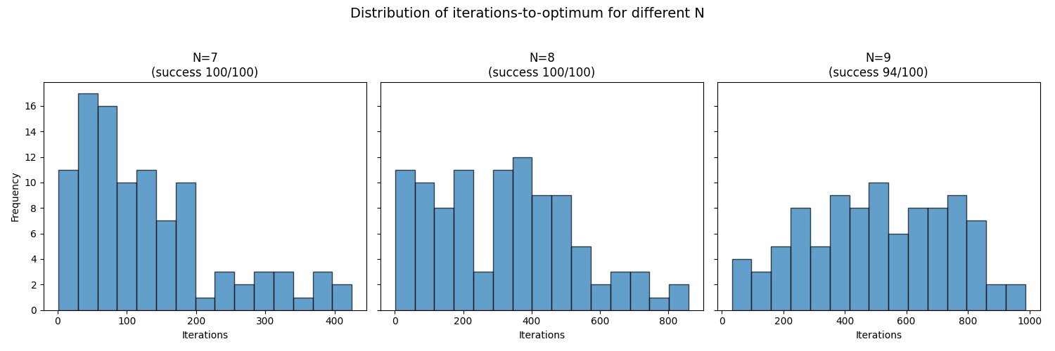
As you can clearly see in the "Distribution of iterations-to-optimum" graph, the results spread out more as the number of cities increases. Let's look at the data:

• For N=7, the algorithm consistently finds the optimal solution (100/100 success rate), and most runs are clustered at a low number of iterations. The average was ~130 iterations (which is in line with what we found in the first graph), but the distribution is wide (std dev: ~104).
• For N=8, the success rate is still 100/100, but the distribution broadens significantly. The average number of iterations more than doubles to ~319, and the spread is much larger (std dev: ~208). Note also, that for our first run we ended up lucky at below 250.
• For N=9, we see a dramatic change. The distribution is even wider (average iterations: ~505, std dev: ~233), and importantly, the success rate drops to 94/100, since we cut off the bell curve at the right side due to the limitation of iterations.

Key Insights

This shows the probabilistic behavior of simulated annealing in action. For smaller problems, it's both fast and reliable. But as the problem scales, two things happen: the number of iterations required to find the optimal solution increases, and the guarantee of finding that solution at all begins to decrease. The algorithm's performance is not a fixed number but a distribution of possibilities, perfectly highlighting the trade-off between speed and certainty.

‍

2. The Convergence Curve

Now that we have investigated the scaling, let's zoom in for a moment on an individual run and the number of iterations.

‍

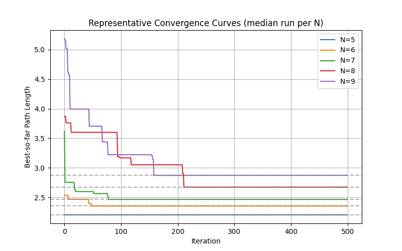
The above graph shows the "convergence" of the annealing algorithm, so how it optimizes over time.

In the example we picked one curve for each network size (N=5 to N=9). On the x-axis we scale up the iteration number of the algorithm and on the y-axis we plot the path length of the current best guess optimization we reach with the algorithm. The gray dashed lines indicate the optimum, which we find using the brute-force approach.

Each line shows the algorithm's progress on a typical run. It starts with a random, high-energy (inefficient) path and, as it iterates, it finds better and better solutions, causing the path length to drop in steps. This visualizes the algorithm intelligently exploring the problem and settling on a low-energy solution.

An interesting detail to notice in the convergence graph is that the run for 8 cities took longer to find its best solution than the run for 9 cities.

This might seem counterintuitive, but it's a perfect illustration of how heuristic algorithms like simulated annealing work. The algorithm starts with a random path and explores the possible solutions randomly.

• In the N=9 case, the algorithm was likely "lucky" and started with a better initial path or found a more direct route to an excellent solution.
• In the N=8 case, it was a bit "unlucky" and likely had to explore more possibilities before it found the best path.
• In the N=7 case, the median run experienced a prolonged local plateau (around ~368 iterations) before making its final drop to the optimum, a classic characteristic of simulated annealing escaping local minima.

This variability is a key characteristic of probabilistic methods. While they are incredibly efficient on average, the performance on any single run can vary due to the random nature of the search. This is another part of the trade-off: in exchange for incredible speed, we accept a small amount of unpredictability in the path the algorithm takes to find the solution.

3. The Success Rate

While the algorithm succeeds reliably when given up to 1,000 iterations, real-world applications often operate under fixed time budgets.

From this perspective it make sense to estimate the success rate given a specific number of iterations and observe how it scales as a function of nodes in the network. This is what we explored in the graph below. On the horizontal axis, we increase the number of nodes (N), while on the y-axis we observe the success rate (how many runs reach the optimum), while we are fixing the number of iterations the algorithm gets to run.

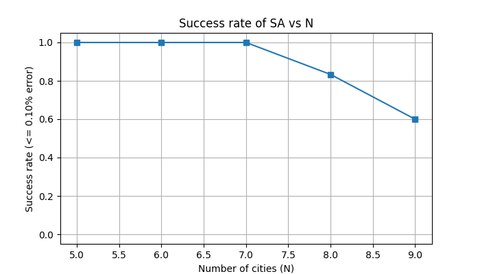
Before we observed that for 1000 iterations, only at N=9 we see the error to appear. The story changes if we limit the iterations to 500:

• For 5, 6, and 7 cities, the success rate remains 100%.
• For 8 cities, the success rate drops to 83.3%.
• For 9 cities, it falls to 60%.

This is the fundamental limitation in action. While simulated annealing is incredibly fast, its guarantee of finding a near-perfect solution diminishes as the problem's complexity grows. This is the reason why, for the world's most complex problems, we must eventually turn to a new form of computation.

While simulated annealing is incredibly efficient, it has one crucial limitation: it works with probabilities and is not guaranteed to find the absolute best solution.

Because the algorithm uses a random process to explore the problem, its success often depends on having enough iterations (tries) to find a good path.

• If the number of iterations is too low, the algorithm may not have enough time to escape a poor solution, leading to an absurd or inefficient result.
• Even with many iterations, it is designed to find a very good solution, known as a local minimum, but it might not find the single best solution, the global minimum.

‍

This trade-off is key: simulated annealing sacrifices the guarantee of perfection for a massive gain in speed.

We encourage you to experiment with this yourself. The code used for these simulations will be made available in the appendix. Running the code and seeing the results firsthand is a fantastic way to solidify your understanding of these concepts.

Where This Leaves Us

So here's where the classical toolbox runs out. Brute force gives us certainty but no scalability. Simulated annealing (like other common methods in today's classical algorithmic toolkit) gives us speed, but no guarantee. All of this becomes very complex and limited, as we try to apply this to real world logistics problems, where we're (depending on the application) talking about hundreds or thousands of stops rather than 9 or 10.

That's the wall we've been building toward across this whole series. In Part 4, we'll step away from classical shortcuts entirely and look at how quantum computer approaches the same problem, mapping our cities and distances onto a quantum energy landscape, and letting the system settle into its lowest-energy state rather than searching for it.

‍

Written by Dhruv Sachdeva and Dr. Jonas Kölzer
‍

‍