
Clearing the Traffic: A Classical Solution to an Impossible Problem
Introduction
In our last article, we explored the vast world of logistics and the massive, NP-hard challenge at its heart: the Traveling Salesperson Problem (TSP). We discovered that as the number of cities increases, the number of possible routes explodes exponentially. This "combinatorial explosion" makes the straightforward brute-force method, checking every single path, completely impractical for real-world scenarios.
So, if brute force fails, how do we find an efficient route? We turn to a much smarter approach: heuristic algorithms.
These are advanced classical methods that use clever shortcuts to find excellent solutions without checking every possibility. For this article, we're going to explore one of the most powerful and fascinating heuristics: simulated annealing.
This method is about intelligently guiding a system to its lowest energy state, or "ground state." That might sound complicated, so let's break it down with an analogy. Think about learning mathematics. You don't jump straight to advanced calculus on your first day. Instead, you start with basic arithmetic and gradually build your knowledge over time, allowing you to solve complex problems easily.
Simulated annealing works similarly. It starts with a random, high-energy solution and slowly "cools" it down, making small, intelligent adjustments at each step. This gradual process allows it to find an excellent, low-energy solution without having to waste time checking every single possibility, making it significantly more efficient than the brute-force method.
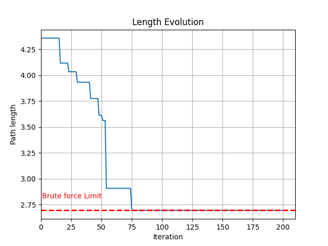
This "Length Evolution" graph is a perfect visual of the algorithm in action:
- The Y-axis (Path length) represents the "energy" (or in logistics the length of the path) of the solution, lower is better.
- The X-axis (Iteration) is time.
- The Blue Line shows the algorithm "learning." It starts with a random, high-energy path (a long, inefficient route). As it "cools" over time, it makes intelligent adjustments, finding better and better solutions, which you see as the steps going down.
- The Red Line ("Brute force Limit") is the perfect, optimal solution found by the brute-force method.
This graph clearly shows the algorithm's intelligent descent, eventually settling on a solution that is extremely close to the perfect "ground state." It’s the visual proof of the "cooling" process we just described.
The Results: A Data-Driven Comparison
You may notice that we're about to look at several different examples, and you might be wondering why. We did this intentionally to see how these algorithms perform under different conditions, by tweaking the number of cities or the number of iterations. This hands-on approach is the best way to build a clear and decisive understanding of their strengths and limitations.
After all, what better way is there to learn than by seeing it in action?
The Scaling Showdown: 5 vs. 8 Cities
Let's start by looking at how the two methods scale. We ran simulations to compare brute-force and simulated annealing on a standard laptop:
- For 5 cities, the brute-force method is incredibly fast, finding the optimal solution in just 1.4 millisecons. At this small scale, brute force is the clear winner, as the annealing algorithm actually takes slightly longer (3 milliseconds to 26 milliseconds).
- However, for 8 cities, the situation changes dramatically. This dramatic change is a direct result of the "combinatorial explosion." The brute-force method still finds the perfect solution, but its execution time explodes to 0.1879 seconds (188 milliseconds), over 130 times longer.
- The simulated annealing method, in contrast, also finds the perfect solution but does so in a mere 2.9 to 29.1 milliseconds, remaining incredibly fast.
Note: The range that we are providing for the simulated annealing is the statistical distribution we observed it took the algorithm to reach the steady ("cooled down") state. This may not always be the optimal solution, as we are talking about an heuristic algorithm rather than a optimal solution finder.
The "11-City" Challenge: An Even Starker Difference
To see just how wide this performance gap gets, let's look at the results for 11 cities:
- Brute-Force Method: It found the perfect solution by checking all 3,628,800 paths, which took 70.05 seconds.
- Simulated Annealing Method: It started with an inefficient path and found the exact same perfect solution in just 5 milliseconds.
Note: This is of course just one example, it does not always have to end of at the perfect solution.
The Key Takeaway
The results are staggering. For a real-world problem, the simulated annealing algorithm found the optimal solution over 13,000 times faster than the brute-force method.
This is where the trade-off becomes clear: while brute-force guarantees the perfect answer, its runtime quickly becomes impractical. Simulated annealing, on the other hand, provides an excellent (and in this case, perfect) solution in a fraction of the time, making it a far more efficient approach. What a great invention of Mother Nature :)
The graphs below illustrate this dramatic difference in performance. You can clearly see the execution time for the brute-force method (blue) skyrocketing, while the time for the simulated annealing algorithm (orange) remains almost flat.

This brings us to some pretty important questions, which require our proper attention:
We've seen that simulated annealing is fast, but how does it truly scale?
What is its breaking point?
And what about its reliability?
We traded the guarantee of a perfect solution for speed, but what are the consequences of that trade-off?
These are critical questions that we must answer. In our next article, we're going to do a deep dive to truly decode the nature of this powerful algorithm. We'll run more detailed experiments to uncover its scaling behavior and see if it's really the ultimate solution.
Join us in Part 3 as we explore the absolute limits of classical heuristics and look to the quantum realm.
📚 References & Further Reading
For those interested in digging deeper into the concepts we discussed, here are a few resources:
- Simulated Annealing: What is Quantum Annealing?, How The Quantum Annealing Process Works
- The Traveling Salesperson Problem (TSP): https://en.wikipedia.org/wiki/Travelling_salesman_problem
- NP-Hard Problems: P vs. NP - An Introduction
Our GitHub Repository: Github
Written by Dhruv Sachdeva and Dr. Jonas Kölzer